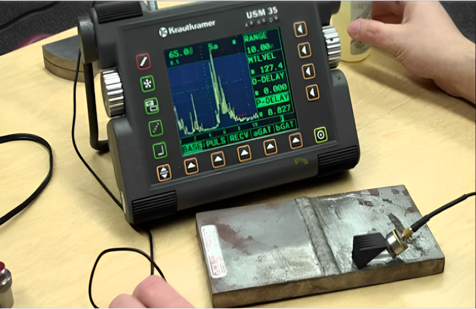
When developing the in-line inspecition robot to measure wall thickness of carbon steel pipes using ultrasonic probes, we encountered a lot of noise affecting the signal. The noise came from the electric motors used to drive the tool through the pipe, structural noise from the carbon steel cavity resonance, and the cables acting as mini antennas due to their long lengths. The below is an example of modeling the signal, noise, and showing how effective a simple band-pass filter can be.

Generating the Signal

A UT is typically a short pulse followed by a series of echos. These echos are the signal being reflected back to a receiver (off a wall or defect). We can generate an ideal noise-free signal by creating a pulse, along with a lower-amplitude pulse that has been time-shifted to represent the reflection of a back wall:

import numpy as np
import matplotlib.pyplot as plt

# create the clean UT signal 
sample_rate = 50e6
time = np.arange(0, 10e-6, 1/sample_rate)
ut_frequency = 5e6

# sine pulse with a Gaussian envelope
def create_pulse(t, delay, amplitude):
    pulse = np.sin(2 * np.pi * ut_frequency * (t - delay))
    envelope = np.exp(-((t - delay)**2) / (2 * (0.2e-6)**2))
    return amplitude * pulse * envelope

def plot_signal(time, signal, title, color='blue'):
    plt.figure(figsize=(12, 4))
    plt.title(title)
    plt.plot(time * 1e6, signal, color=color)
    plt.xlabel("Time (μs)")
    plt.ylabel("Amplitude")
    plt.grid(True)
    plt.show()

main_bang = create_pulse(time, 2e-6, 1.0)
echo = create_pulse(time, 5e-6, 0.4) # from back wall

clean_signal = main_bang + echo

plot_signal(time, clean_signal, "Simulated Clean UT Signal", "red")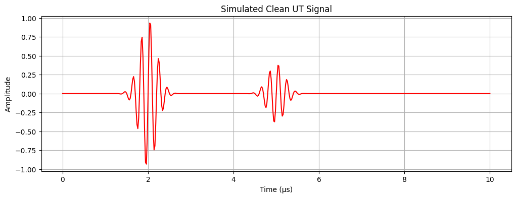

Now this won’t look anything like a UT signal if you’ve worked with UT machines, and that’s because there’s post-processing done to the signal so that it’s easier to interpret.

What UT probes normally show is a trace of the amplitude of the pulse - we can show this using the Hilbert transform. It’s useful for automatic peak detection algorithms.

from scipy.signal import hilbert

envelope_signal = np.abs(hilbert(clean_signal))

plot_signal(time, envelope_signal, "Smoothed UT Signal Envelope")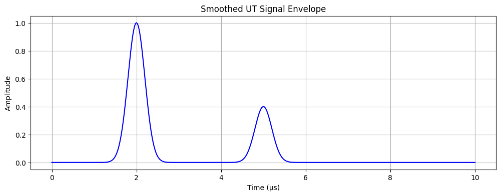

Now that we have the ideal signal, let’s see what it looks like with noise present.

# noise from a nearby motor
motor_noise_freq = 50e3
motor_noise = 0.3 * np.sin(2 * np.pi * motor_noise_freq * time)

# general broadband noise
random_noise = 0.2 * np.random.randn(len(time))

noisy_signal = clean_signal + motor_noise + random_noise

noisy_envelope_signal = np.abs(hilbert(noisy_signal))

plot_signal(time, noisy_envelope_signal, "Smoothed UT Noisy Signal Envelope")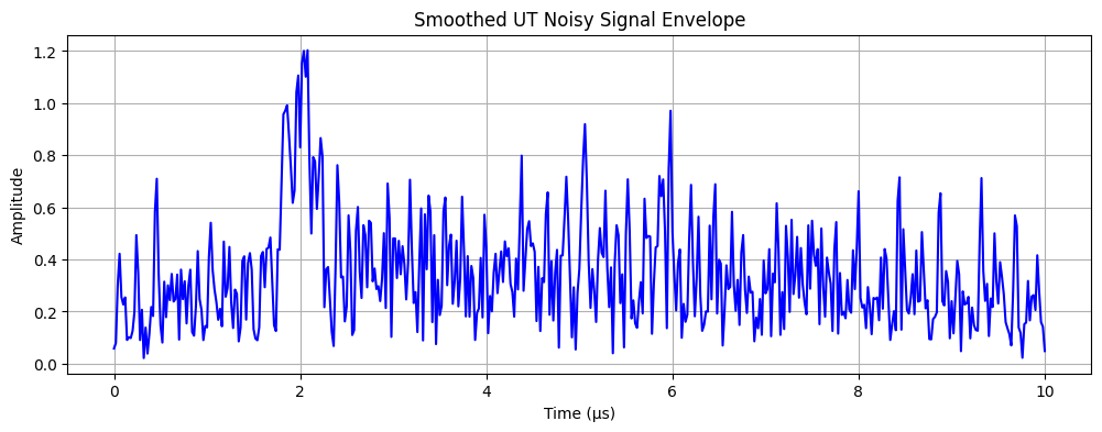

You’ll notice we now completely lose the signal of the echo. Since we know the frequency of the UT signal (it can be set by the technician on nearly all UT machines), we can design a band-pass filter to only pass frequencies around our UT signal.

from scipy import signal

# band-pass filter (Butterworth) passing frequencies around our 5 MHz UT signal
b, a = signal.butter(4, [4e6, 6e6], btype='bandpass', fs=sample_rate)

filtered_signal = signal.lfilter(b, a, noisy_signal)

noisy_filtered_envelope_signal = np.abs(hilbert(filtered_signal))

plot_signal(time, noisy_filtered_envelope_signal, "Smoothed UT Filtered Signal Envelope")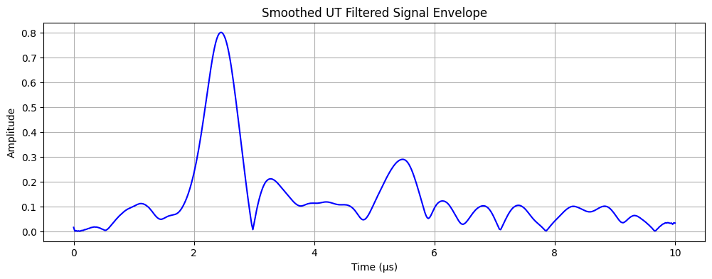

It’s important to consider how this filter could be implemented. UT probes can change the frequency, so creating a passive filter likely wouldn’t work unless the band allowed is large enough to cover the possible range of frequencies. An active digital filter would be ideal but requires more computation resources.

More could be done to improve the signal. Some things I would like to try tackle later:

• Build a 3D model and look into more realistical signals using something like OnScale
• A more realistic model, specifically to take into account strucural noise caused by signals bouncing around the carbon steel pipe as well as the UT cable acting as a mini antenna to take into account electromagnetic interference (EMI).